From Research Intuition to 1.21 bpb: My Parameter Golf Journey

Opening

When I first looked at OpenAI’s Parameter Golf challenge, I did not see it as just another benchmark to optimize against. I saw it as a compressed systems problem with prediction at its core. Given my past experience with prediction-focused modeling, my mind immediately went to Markov chains as a possible starting point.

That was what made it interesting.

The goal was not simply to train a smaller model. The goal was to find a way to preserve as much predictive power as possible under hard boundaries on size, time, and compute. In practice, that meant every architecture choice, every compression decision, every training knob, and every evaluation detail had to justify its existence.

What made this journey personal for me is that the core idea did not start with language models. Years earlier, during my undergraduate research, I was already exploring prediction-oriented modeling and structured sequential behavior. Looking back at some of that work, I can see the same instinct that later resurfaced in Parameter Golf: the belief that local transitions can still carry meaningful predictive signal, even inside more complex systems.

That earlier work was not about modern language modeling, but the underlying questions were related: how do you represent sequential structure, how do you capture useful local relationships, and how do you turn noisy observations into something predictive?

Even in that earlier work, I was already thinking in procedural terms about calibration, node relationships, and how local signal structure might be turned into a usable predictive mechanism. The implementation in Parameter Golf was very different, of course, but the intuition behind trying a Markov-style direction felt familiar.

Parameter Golf became the perfect place to test that intuition in a modern form.

The Starting Point: Why Markov at All?

A lot of language modeling work defaults to the assumption that more transformer capacity is the right answer as long as the budget allows it. In this challenge, though, the budget was the whole game.

That changed the framing.

Instead of asking, “How do I build the best transformer I can?” the more useful question became, “What information can be captured cheaply, and what information actually needs transformer capacity?”

That was the opening for the hybrid idea.

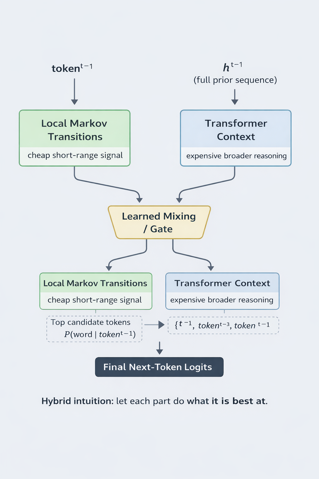
Local token transition structure is not enough to solve language modeling on its own, but it is also not meaningless. There are many places where short-range statistical regularities still matter. If some of that can be captured explicitly by a lightweight Markov-style component, then the transformer may be able to spend its limited capacity on broader contextual reasoning instead of relearning every local regularity the expensive way.

That became the working hypothesis: blend a causal GPT with an explicit Markov component and make the combination size-efficient enough to survive the competition constraints.

Early Direction

The broad direction was a GPT-style model with a Markov signal blended into the logits. But broad direction is cheap; the hard part is making something like that actually work under competition constraints.

There were several practical questions right away:

• How large should the transformer backbone be?
• How should the Markov signal be represented?
• Should the Markov side be static, learned, gated, or confidence-aware?
• How do you quantize aggressively without collapsing performance?
• How do you fit everything into the artifact limit after compression?
• Which improvements are real and which ones are just noise from small evaluation differences?

Those questions led to a long series of experiments rather than one clean jump to the final design.

The Experiment Loop

A lot of the real work was not glamorous. It was repeated iteration under time pressure.

I tested scale changes from 9 layers to 10 layers to 11 layers. I compared quantization schemes, compression strategies, KV head counts, initialization choices, and different ways of using Markov-style structure. I also explored both 1st-degree and 2nd-degree Markov attempts before settling on the final direction. Some ideas looked promising in theory and just did not pay off at this training budget. Others helped a little but not enough to justify the bytes they consumed.

A few examples from the path:

• Scaling from 9L to 10L to 11L
• Testing EMA, which turned out to be harmful here
• Testing QAT, which was also harmful at this step count
• Comparing int8 against mixed int6/int8 quantization
• Comparing zlib against zstd compression
• Increasing batch size from 524K to 786K tokens
• Sweeping mix initialization values
• Trying bigram hash caches
• Comparing 2 versus 4 KV heads

This was one of those projects where “good idea” and “good idea under this exact constraint set” were often very different things.

The Architecture I Ended Up With

The strongest version that emerged was an 11-layer, 512-dimensional GPT with adaptive Markov mixing and mixed int6/int8 quantization.

At the architecture level, the model used:

• 11 transformer layers
• 512 hidden dimension
• GQA with 8 attention heads and 4 KV heads
• Tied embeddings
• ReLU-squared MLPs
• U-Net-style skip connections
• RoPE positional encoding

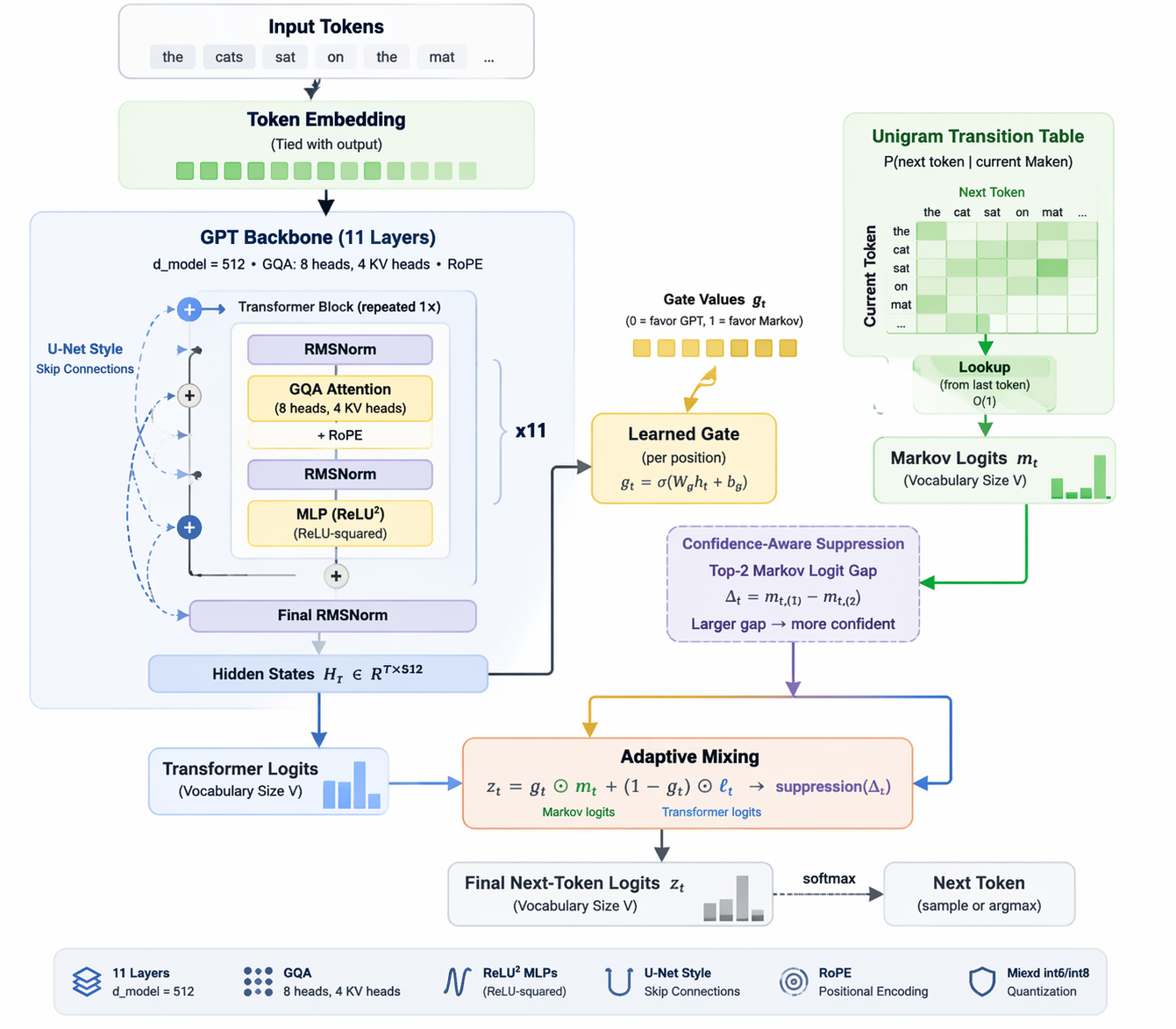
The hybrid piece came from blending transformer logits with a unigram transition table using a learned per-position gate derived from the hidden state. The Markov side was not treated as a universal answer; it was one signal among others.

To make the blend more selective, I also used a confidence-aware mechanism based on the top-2 Markov logit gap. That allowed the Markov contribution to be suppressed when the transformer appeared more trustworthy, instead of forcing the hybridization equally across all positions.

That mattered because the goal was never to let the Markov side dominate. The goal was to let it help when local transition structure was informative and stay out of the way when broader context mattered more.

Compression Was Not an Afterthought

One of the biggest lessons from Parameter Golf is that compression is not a post-processing step. It is part of the modeling strategy.

If your architecture only works before the artifact limit is enforced, then it does not really work for the competition.

The final approach used mixed quantization:

• MLP and attention weights used per-row int6 quantization
• embeddings and the Markov table used int8
• small control tensors stayed in fp16 where needed

The int6 values were clamped to the target range and stored in int8 containers. That sounds wasteful on paper, but in practice zstd at a high compression level recovered much of that wasted space. In other words, the storage format and the compressor had to be thought about together.

That kind of detail ended up mattering a lot. It was not enough to ask whether int6 or int8 was better in isolation. The right question was which representation produced the best end-to-end tradeoff once quantization error, storage layout, and final compression were all taken into account.

Training Under the Clock

The challenge environment forced a very specific style of thinking. You do not get the luxury of endless training and late-stage cleanup. You need a model that becomes competitive fast.

The final run used a 786K-token global batch on 8xH100 and processed about 5.84 billion tokens in roughly 600 seconds, reaching around 7,430 steps within the time cap.

That meant every training decision had to be judged by whether it helped inside that narrow window, not whether it might help eventually.

This is also why some common ideas did not survive. EMA and QAT are both reasonable techniques in many settings, but at this budget and step count they were net negative. Parameter Golf was a good reminder that a method being broadly valid does not mean it is valid for a short-horizon, compression-constrained race.

Where I Landed

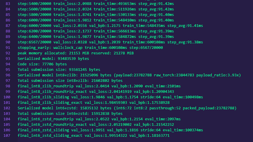
The main PR ultimately landed at:

• 1.2171 mean val_bpb
• standard deviation of 0.0003 across 3 seeds
• compressed artifact size around 14.9 to 15.1 MB

That result came from a lot of iteration, a lot of pruning, and a lot of refusing to treat any single component as sacred.

Later runs suggested that the hybrid still had more headroom, with follow-up experiments pushing into the 1.18 range under the same broader line of attack.

That created a strange dynamic: part of the project was no longer just about finding the next improvement, but about waiting to see where the earlier PR would officially land so I could judge how hard it still made sense to push.

What This Project Reinforced for Me

A few things became clearer through this challenge.

First, hybrid modeling still has room to surprise people. Not every gain has to come from scaling the same architecture family harder. Sometimes a carefully chosen cheap signal can genuinely complement a more expressive model.

Second, systems thinking matters just as much as model thinking. Architecture, quantization, training dynamics, serialization, and compression all interact. Treating them as separate phases leaves performance on the table.

Third, constraint-heavy competitions expose what is actually robust. Ideas that sound impressive in the abstract get filtered quickly when they have to survive a wall-clock cap and an artifact-size cap at the same time.

And finally, this was a reminder that old research intuitions can come back in useful ways years later. The Markov angle was not something invented just to look clever for a benchmark. It came from a much older fascination with sequential structure and prediction in noisy systems. Parameter Golf simply gave that instinct a modern battlefield.

Closing

What I liked most about this journey is that it did not feel like blindly turning knobs. It felt like building toward an idea, testing it honestly, and then forcing it to earn its place under real constraints.

That is a satisfying kind of work.

Whether the takeaway is the exact hybrid architecture or just the broader lesson that cheap local structure can still be worth modeling explicitly, I think the challenge was a great example of why constrained optimization problems are so valuable. They force clarity.

And in this case, that clarity led from an old research instinct to a modern compressed model that could actually compete.

Earlier Markov Attempts

Before landing on the final adaptive unigram-mixing approach, I spent real time exploring both 1st-degree and 2nd-degree Markov variants.

The 1st-degree direction was the most natural starting point. It kept the representation relatively simple and made it easier to test whether explicit local transition structure was helping at all once combined with GPT logits.

The 2nd-degree direction was appealing for a different reason: in theory, it could capture a richer short-range signal by conditioning on a slightly deeper local history. But Parameter Golf is ruthless about bytes, implementation complexity, and what actually survives short training windows. Even when an idea is directionally promising, it still has to earn its place under compression and runtime constraints.

Those earlier attempts were not wasted detours. They were part of how I arrived at the final design. They helped me see that the most useful version of the Markov idea in this competition was not necessarily the most elaborate one, but the one that gave the best end-to-end tradeoff once modeling value, quantization, compression, and artifact size were all considered together.

Appendix: Concise Technical Summary

• 11-layer, 512-dim GPT
• Adaptive Markov mixing via learned per-position gate
• Confidence-aware suppression using top-2 Markov logit gap
• GQA: 8 heads, 4 KV heads
• Tied embeddings, ReLU-squared MLPs, U-Net skip connections, RoPE
• Mixed int6/int8 quantization
• zstd-22 compression
• 786K-token batch, 5.84B tokens total, ~7,430 steps in 600s on 8xH100
• Final main result: 1.2171 mean val_bpb over 3 seeds, ~15MB artifact