A Hands-On Exploration with Gemma 3 1B PT

When people discuss model compression, the focus often jumps immediately to production systems, benchmark tables, or highly optimized quantization libraries. I wanted to approach it differently.

Rather than beginning with a black-box tool and accepting its output at face value, I wanted to understand what compression is actually doing to a model. My interest was not only in reducing size, but in building intuition for a broader question: how might we eventually fit models that seem too large for a given GPU or hardware constraint? Answering that requires looking below the surface at the mechanics of quantization, compression, and how predictive behavior shifts when parts of a network are altered at a low level.

That curiosity led me to a simple starting point: why not try 2-bit quantization?

To explore that, I built a basic 2-bit quantization pipeline, applied it to a real open-weight model, and examined how the model’s behavior changed as different components of the network were perturbed.

In this article, I walk through the model and tools I used, why I chose them, how the experiment was structured in code, and what I observed while quantizing parts of Gemma 3 1B PT.

The Goal

The original goal was simple:

Could I manually compress parts of an open language model toward 2-bit representations and observe how the model’s behavior changed?

This was not a production quantizer and not an attempt to beat established compression libraries. It was an exploratory experiment meant to answer questions like:

• What does a model tensor actually look like?
• How much can a single tensor be distorted before generation changes?
• Are some parts of a transformer more sensitive than others?
• Does lower reconstruction error automatically mean less behavioral drift?

That last question turned out to be especially important.

Why Gemma 3 1B PT?

I downloaded the base model from the official Google Hugging Face repository for Gemma 3 1B PT:

https://huggingface.co/google/gemma-3-1b-pt

I chose Gemma 3 1B PT as the base model for a few reasons.

First, it was small enough to experiment with locally without the project immediately turning into a storage or hardware problem. For a first low-level compression study, I wanted something large enough to be meaningful, but still manageable enough to inspect, modify, and reload repeatedly during testing.

Second, I specifically wanted the pretrained checkpoint rather than the instruction-tuned version. For this experiment, the pretrained model was the cleaner object to study. The goal was not to evaluate assistant-style usefulness or chat alignment, but to observe what happens when the underlying network itself is perturbed. I wanted to see how aggressive 2-bit quantization affected the base model’s raw generation behavior, which parts of the transformer appeared more sensitive, and how compression changed outputs at a more fundamental level.

An instruction-tuned model would have introduced another variable, since its behavior is shaped not only by the pretrained weights but also by additional post-training designed to make it act more like an assistant. That is valuable for real-world use, but less ideal for isolating low-level compression effects.

Third, the local checkpoint structure was simple and easy to inspect. It included a config.json, tokenizer files, and a single model.safetensors file. That made it a practical target for a first-principles quantization experiment.

When I inspected the checkpoint, the model appeared as a network with 340 tensors and just under 1 billion parameters. That was large enough to matter, while still being manageable for targeted experiments.

Step 1: Inspecting the Model

Before compressing anything, I wanted to see what the model was actually made of.

The first inspection script loaded the .safetensors file and printed tensor names, shapes, dtypes, and parameter counts. That made the transformer structure much more concrete and turned the checkpoint from a single opaque file into something I could actually reason about.

A few things became immediately obvious.

At the front of the model was a token embedding matrix, which acts as the lookup table that maps token IDs into dense vectors. In practical terms, this is the model’s first translation layer from discrete tokens into the continuous representation space it uses internally.

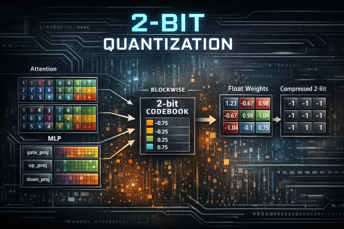
Each transformer block then broke down into two main computational parts: self-attention and the MLP (feedforward) network. The attention side contained the familiar projection matrices:

• q_proj
• k_proj
• v_proj
• o_proj

These are the matrices that let tokens interact with one another. The query, key, and value projections define how tokens search for, match against, and retrieve information from other positions in the sequence, while the output projection maps that attended result back into the model’s main hidden representation.

The MLP side of each block contained another set of large projection matrices:

• gate_proj
• up_proj
• down_proj

These handle the per-token transformation work that happens after attention. In simplified terms, up_proj expands the representation into a larger intermediate space, gate_proj helps control which features are emphasized, and down_proj compresses the result back into the model’s normal hidden size.

By contrast, the LayerNorm-style weights were tiny. They are mostly per-dimension scaling parameters rather than large 2D projection matrices, so they contribute very little to the total parameter count compared with attention and MLP weights.

That naming structure also made it much easier to decide what to perturb. Instead of treating the model as one giant blob of parameters, I could target specific parts of the network in a controlled way:

• a single tensor
• one layer only
• attention only
• MLP only
• multiple adjacent layers

That turned out to be the right way to structure the experiment. Once the checkpoint was decomposed into embeddings, attention projections, MLP projections, and normalization weights, it became much easier to reason about where compression was likely to matter most and where perturbations would be easier to interpret.

Step 2: Building a Simple but Transparent 2-Bit Quantizer

I did not begin with an advanced quantization library or a highly optimized compression pipeline. Instead, I built a deliberately simple blockwise 2-bit quantizer so I could understand every step of the process and inspect the behavior directly.

The goal was not to build the best possible quantizer. It was to build one that was easy to reason about.

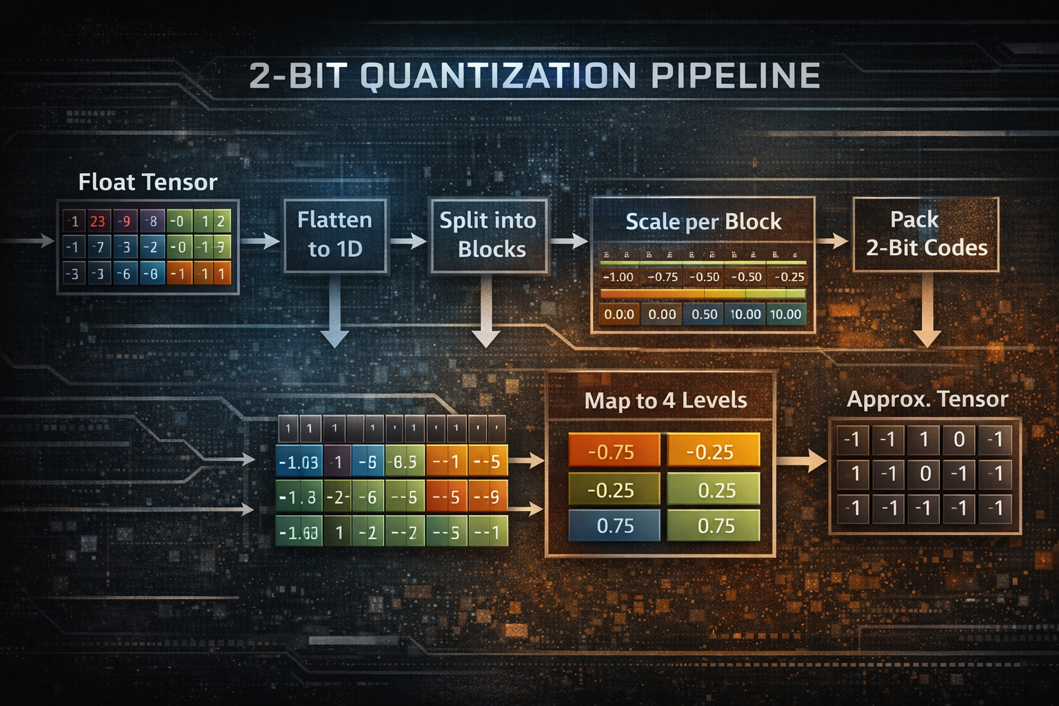
At a high level, the quantization flow looked like this for each tensor:

• flatten the tensor values into a 1D array
• split that array into fixed-size blocks
• for each block:
  • compute a scale from the maximum absolute value
  • normalize the block by that scale
  • map each normalized value to one of four allowed quantization levels
• pack the resulting 2-bit codes into bytes
• reconstruct the tensor by dequantizing those codes back into approximate floating-point values

This design was intentionally simple. I wanted to trace the full path from original weights to quantized representation to reconstructed tensor without hiding the important details behind library abstractions.

In this context, the quantization levels are the small set of values each normalized weight is allowed to snap to. Since 2-bit quantization only provides four possible states, every value in a block must be approximated using one of just four reconstruction values. You can think of these levels as the four buckets available to represent the continuous range of normalized weights.

A weight that originally had a value like 0.18 or -0.82 could no longer be stored exactly after normalization. Instead, it had to be replaced by the closest allowed level, and then reconstructed later by multiplying that level by the block scale. That is the core tradeoff of aggressive quantization: fewer bits and less storage, but also less precision.

This was not designed to be optimal. It was designed to be inspectable.

What the Levels Actually Are

In a quantizer, the levels are the small set of numeric values a real number is allowed to snap to after quantization.

Normally, a tensor weight might be any floating-point value, such as -0.82, 0.14, or 0.67. But with 2-bit quantization, each value only has 2 bits of storage, which means there are only 2^2 = 4 possible states available. That means every normalized weight has to be approximated by one of only four allowed reconstruction values.

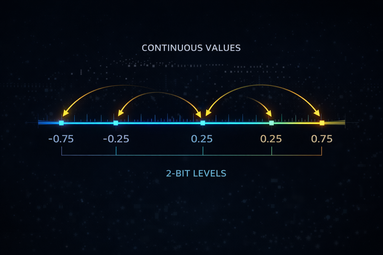
So when I define a level set like:

[-1.0, -1/3, 1/3, 1.0]

I am really saying: after normalization, every value in that block must be replaced by whichever of those four values is closest.

For example, if a normalized weight is 0.20, it might get mapped to 1/3. If it is -0.90, it might get mapped to -1.0. During dequantization, that chosen level is then multiplied back by the block scale to reconstruct an approximate floating-point value.

So the levels are effectively the quantizer’s vocabulary. They define the only values the compressed representation is allowed to express inside each block.

Why Blockwise Quantization?

Using a single scale for an entire tensor is usually too crude. Large weight tensors often contain regions with different magnitude patterns, and one global scale can wash out those local differences.

Blockwise quantization gives each chunk of values its own scale, which makes the approximation more locally adaptive while still keeping the implementation straightforward. It was a useful middle ground: simple enough to inspect, but not so naive that reconstruction quality collapsed immediately.

Why the Quantization Levels Mattered

With 2 bits, there are only four reconstruction states available, so the exact placement of those states matters a great deal.

My initial experiments used a more obvious symmetric set of levels:

[-1.0, -1/3, 1/3, 1.0]

That worked as a starting point, but it quickly became clear that the codebook itself had a major effect on reconstruction quality. In other words, the question was not just how to pack 2-bit values efficiently, but which four values those 2-bit codes should represent in the first place.

For this experiment, the best-performing level set I found was:

[-0.75, -0.25, 0.25, 0.75]

That codebook consistently outperformed the earlier, more naive choices on reconstruction error. Even in a simple 2-bit pipeline, the choice of levels turned out to be one of the most important design decisions.

Step 3: Testing One Tensor First

The first real target was a single attention weight tensor:

model.layers.0.self_attn.q_proj.weight

In this context, a tensor is just a block of numbers arranged in one or more dimensions. A vector is a 1D tensor, a matrix is a 2D tensor, and the large learned weight objects inside neural networks are typically stored as tensors. In this particular case, the tensor was a weight matrix used by the model’s attention mechanism.

That made it a good first test case because it was a real transformer weight object inside the live model, but still small enough to inspect and reason about in isolation.

The script performed four basic steps:

• load the original tensor
• quantize it into the custom 2-bit format
• reconstruct it back into approximate floating-point values
• compare the original and reconstructed values

This was the first point where the experiment moved from designing a quantizer to measuring what it actually did. It gave me the first real compression statistics and reconstruction error metrics on an actual model weight.

What I Learned From the One-Tensor Test

A few things became clear immediately.

First, the custom 2-bit packing pipeline worked. The packing and unpacking stages were exact at the code level, which meant any loss came from quantization itself rather than from a bug in the storage format.

Second, reconstruction error was real, but manageable. The quantized tensor was clearly an approximation of the original, yet it remained close enough to preserve much of the underlying structure.

Third, the choice of codebook mattered more than I initially expected. Small changes to the reconstruction levels produced noticeably different error profiles, which reinforced the idea that even a very simple 2-bit quantizer still has meaningful design choices inside it.

Most importantly, when I swapped the reconstructed tensor back into the live model and generated text from a test prompt, the greedy output stayed identical.

That was one of the first genuinely useful results in the project. It suggested that a single transformer weight matrix could absorb a meaningful amount of quantization noise without visibly changing greedy output.

Step 4: Moving From One Tensor to One Full Block

After the single-tensor test, I escalated to the major linear weight tensors in the model’s first transformer block, or layer 0.

In this context, a block is one full transformer layer: a repeated unit inside the network that contains both the attention sublayer and the MLP sublayer. Earlier I had quantized one tensor in isolation. Now I was quantizing the main learned weight matrices that together make up an entire computational block.

For layer 0, that meant quantizing the major linear weights from both:

• the attention projections
• the MLP projections

This was the first point where the model’s behavior changed dramatically.

What Changed?

The model did not collapse into gibberish. That was important. The output remained grammatical, readable, and structurally coherent.

What changed instead was the model’s behavioral trajectory.

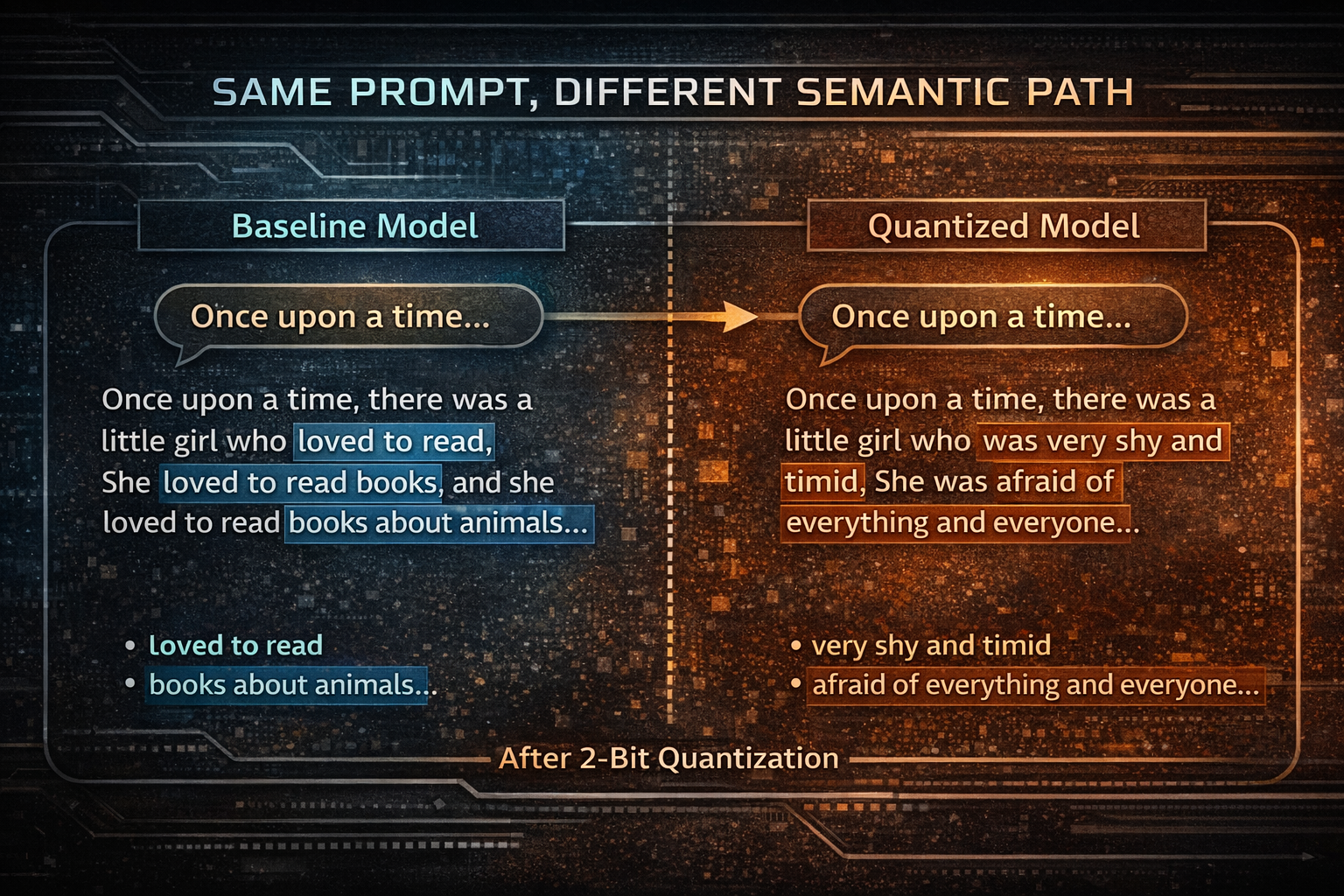
For example, the baseline story prompt began with a little girl who loved reading books about animals, while the layer 0 MLP-only perturbation redirected it into a different story about a girl who was “very shy and timid” and “afraid of everything and everyone.”

The output remained fluent, but it was no longer behaviorally close to the original continuation.

That was a turning point in the experiment.

Up to that point, the question had mostly been whether 2-bit quantization would visibly break the model. But at the block level, a more interesting pattern appeared: the model could remain coherent while still becoming behaviorally different.

This suggested something important. The quantization noise was not just degrading quality in a generic sense. It was pushing the model into different high-probability completion paths, or different local attractors in generation space.

In other words, once enough of a transformer block was perturbed, the result was not necessarily nonsense. It could be a model that still wrote plausible text, but one that had been nudged into behaving like a meaningfully different version of itself.

Step 5: Expanding the Prompt Set

To avoid over-interpreting the behavior of a single prompt, I expanded the test setup into a small prompt suite covering several different styles of continuation:

• story continuation
• factual continuation
• programming explanation
• science-news style continuation
• short math QA

That mattered because a quantized model can appear stable on one prompt while drifting badly on another. A broader prompt set made it easier to tell whether a result was isolated or part of a more general pattern.

I also extended the script so that each test run followed the same sequence:

• run the baseline generation with the original model
• swap quantized tensors into the model
• run generation with the modified weights
• restore the original tensors
• rerun generation
• compare the first divergence point between the baseline and quantized outputs

That made the experiment much more repeatable. Instead of relying on casual eyeballing, I could compare when the outputs first separated and how large the behavioral drift became after the swap.

I also updated the script to write results both to the console and to a text file using a small Tee helper, so each run was documented automatically. That made it much easier to compare experiments across different tensors, codebooks, and prompt styles without losing the output history.

Step 6: The Big Question: Which Parts of the Model Matter Most?

Once the basic quantization and tensor-swapping machinery was working, the experiment became much more interesting.

Up to that point, I had already seen that quantizing a full block could change the model’s behavior. The next question was more specific: which parts of the model were actually driving that change?

To answer that, I split the perturbations more carefully.

A transformer is built from a stack of repeated layers, also called blocks. Layer 0 refers to the first transformer block in the network, layer 1 refers to the second, and so on. Each layer contains two major computational parts: the attention sublayer and the MLP sublayer.

When I say attention only, I mean I quantized only the attention projection weights in that layer, such as q_proj, k_proj, v_proj, and o_proj, while leaving the MLP weights untouched.

When I say MLP only, I mean I quantized only the feedforward projection weights in that layer, such as gate_proj, up_proj, and down_proj, while leaving the attention weights untouched.

So instead of perturbing an entire layer all at once, I could isolate which subcomponent was responsible for more of the behavioral drift.

I tested:

• layer 0 attention only
• layer 1 attention only
• layer 0 MLP only
• layer 1 MLP only
• layers 0 and 1 attention only
• layers 0 and 1 MLP only
• layers 0 and 1 full

This mattered because the attention and MLP parts of a transformer block do different jobs. Attention controls how tokens interact with one another across the sequence, while the MLP performs deeper per-token transformation after that information has been mixed. By perturbing them separately, I could start to see whether one side was more behaviorally fragile than the other.

The result was not a precise scientific ranking, but it did produce a rough behavioral sensitivity map. It showed which perturbations caused small drift, which caused larger divergence, and which combinations seemed to redirect generation most strongly.

What the Results Suggested

1. Lower Reconstruction Error Did Not Guarantee Smaller Behavioral Changes

This was one of the most important findings in the experiment.

Some perturbation sets produced lower average reconstruction error than others, yet caused earlier or more substantial changes in generation. In other words, a tensor group could look better under a simple metric like mean squared error while still pushing the model further away from its original completion path.

A particularly clear example came from layer 0. The attention-only perturbation had an average MSE of 0.00011169, while the layer 0 MLP-only perturbation had a lower average MSE of 0.00008584. Despite that, the MLP-only case produced a much stronger semantic shift in generation.

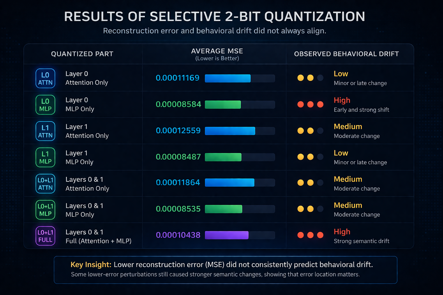
That suggested a key point: where the error lands matters as much as how much error there is. Quantization error is not behaviorally uniform. Small changes in more sensitive parts of the network can matter more than larger changes in less sensitive ones.

2. MLP Perturbations Were Often More Behaviorally Disruptive Than Attention Perturbations

When I split the experiment into attention-only and MLP-only perturbations, the MLP side usually caused stronger semantic drift.

Attention perturbations often kept the model closer to its original trajectory for longer, even when the output eventually diverged. MLP perturbations, especially in earlier layers, were more likely to redirect the model into a different semantic trajectory entirely.

For example, in the layer 0 attention-only run, the story prompt remained identical over the visible excerpt, while other prompts drifted more through repetition than full topic redirection. In the layer 0 MLP-only run, the same story prompt shifted into a substantially different continuation almost immediately.

That was an important pattern, because it suggested that the feedforward side of the block may be more behaviorally fragile under aggressive low-bit perturbation than the attention side, at least in these tests.

3. Layer 0 MLP Was Especially Sensitive

The strongest single-component case I tested was:

• layer 0 MLP only

Even though its reconstruction error was not dramatically worse than some other cases, its effect on output was strong and often appeared early.

That suggested the MLP in the first transformer block may play an outsized role in stabilizing the model’s initial semantic trajectory. Once that part was perturbed, the model often remained fluent, but it was much more likely to head in a meaningfully different direction.

4. Layer 0 Attention Was Comparatively Robust

The least disruptive case I tested was:

• layer 0 attention only

Some prompts stayed identical under that perturbation, which was not true for several of the MLP cases.

That does not mean the attention weights were unimportant. It means that, in this experimental setup, perturbing the first layer’s attention projections alone often produced less immediate behavioral drift than perturbing the first layer’s MLP weights.

5. Two-Layer Full Perturbation Compounded the Drift

The strongest full perturbation case I tested was:

• layers 0 and 1
• mode: full
• block size: 32
• levels: [-0.75, -0.25, 0.25, 0.75]

This produced the clearest multi-prompt behavioral drift while still preserving fluency. The model did not collapse into unreadable output. Instead, it stayed grammatical while drifting toward repetitive, boilerplate-heavy, or factually strange continuations.

The aggregate error for that run was still modest by simple numeric standards, with an average MSE of 0.00010438 and a worst max absolute error of 0.16210938, yet the behavioral drift across prompts was clear.

That was one of the most interesting outcomes in the project: the compressed model could still sound like a language model, yet no longer behave like the same one.

Example Output Shifts

To make those behavioral differences more concrete, it helps to look at a few representative excerpts from the actual runs.

Example 1: Story Continuation Under Layer 0 MLP Perturbation

For the prompt:

Once upon a time

the baseline continuation began as:

“Once upon a time, there was a little girl who loved to read. She loved to read books, and she loved to read books about animals...”

Under the layer 0 MLP-only perturbation, it shifted to:

“Once upon a time, there was a little girl who was very shy and timid. She was afraid of everything and everyone...”

This was one of the clearest cases where the output remained fluent and grammatical, but the model clearly stopped behaving like the same continuation engine.

Example 2: Factual Continuation Under Attention Perturbation

For the prompt:

The capital of France is

the baseline continuation began as:

“The capital of France is a city of contrasts. It is a city of history, culture, and art...”

Under layer 1 attention-only perturbation, the continuation drifted into repetitive self-rephrasing:

“The capital of France is a city of contrasts. It is a city of contrasts in the sense that it is a city of contrasts...”

This was useful because it showed a different failure mode. The model did not jump topics entirely. Instead, it stayed locally fluent while falling into a repetitive attractor.

Example 3: Programming Continuation Under Two-Layer MLP Perturbation

For the prompt:

Python is a programming language that

the baseline continuation framed Python as a language used for “a wide range of applications.”

Under the layers 0 and 1 MLP-only perturbation, the continuation narrowed into a more repetitive description centered on “scripting and data processing.”

That mattered because it was not obvious gibberish. It was plausible text, but behaviorally narrower and less faithful to the original continuation path.

Taken together, these examples reinforced the broader pattern in the experiment: aggressive low-bit perturbations often preserved surface fluency while changing the semantic direction, stability, or repetitiveness of the generated text.

The Code Structure I Used

The final experiment harness ended up with a few main components.

1. Target Selection

I built a helper that took:

• a list of target layers
• a target mode: attention, mlp, or full

and automatically constructed the corresponding tensor names.

That made it easy to run experiments such as:

• [0] + mlp
• [1] + attention
• [0, 1] + full

without hand-editing tensor names every time. More importantly, it made the experiments easier to scale and repeat. Once the selection logic was parameterized, I could move from one-off tests to more systematic sweeps across different parts of the network.

2. Blockwise Quantization and Reconstruction

The quantizer itself used:

• block splitting
• per-block scales
• a fixed 4-level codebook
• dequantization back into float tensors

This part was intentionally simple. The point was not to maximize compression quality, but to make the entire process transparent and easy to modify. Because the quantizer was small and inspectable, I could change block size, codebook levels, or reconstruction logic without fighting a larger abstraction layer.

3. In-Model Swapping

The experiment did not stop at reconstruction error. It actually replaced live model parameters with reconstructed tensors and then ran generation directly.

That was the step that turned the project from a numeric compression test into a behavioral one. Measuring error statistics alone can tell you how much a tensor changed, but not what those changes mean for the model’s outputs. Swapping reconstructed weights back into the live model made it possible to test the thing that ultimately mattered most: how the model behaved after quantization.

4. Prompt Suite Runner and Diff Summary

I added logic to:

• run a prompt list automatically
• compare baseline, swapped, and restored generations
• report the first divergence index

This made the results much easier to interpret. Instead of manually scanning outputs and guessing where a perturbation mattered, I had a repeatable way to see when the quantized model first diverged from the baseline and how that divergence evolved across different prompt types.

5. Output Logging

Finally, I added file logging so every run was saved as a text artifact.

That turned out to be more useful than I expected. Once the experiment space started growing across layers, modes, block sizes, and codebooks, having a persistent record of each run made comparisons much easier and helped keep the results reproducible.

Why This Was Worth Doing by Hand

There are already powerful quantization tools available, so it is reasonable to ask why I went through the trouble of building this manually.

The answer is that building it by hand exposed things a black-box workflow tends to hide.

This experiment made several ideas much more tangible:

• tensors are just named blocks of learned numbers
• codebooks matter
• block size matters
• average reconstruction error is not the whole story
• different transformer submodules are not equally sensitive
• behavior can change dramatically even when the model remains fluent

That last point was probably the most interesting.

The model often did not become “broken.” It became different.

And that difference was not random noise. It had structure. The model could remain grammatical, locally coherent, and superficially plausible, while still being redirected into a noticeably different semantic trajectory. That is a much more interesting failure mode than simple collapse, because it suggests that aggressive quantization can preserve surface fluency while changing the deeper behavioral character of the model.

What I Would Do Next

If I continued this line of work, the next steps I would be most interested in are the following.

1. Token-Level Divergence Tracking

In the current experiment, I measured the first divergence index at the character level. A cleaner next step would be to track divergence at the token level instead, which would align the analysis more closely with how the model actually generates text.

2. More Systematic Submodule Sensitivity Mapping

I now have a useful starting point across:

• layer 0 vs. layer 1
• attention vs. MLP

The next step would be to push that analysis deeper into the stack and build a broader sensitivity map across more layers and tensor families.

3. Better Codebooks

The current quantizer was intentionally simple, which leaves plenty of room for improvement. Some obvious next directions would be:

• asymmetric codebooks
• learned codebooks
• zero-centered variants
• data-driven level choices for different tensor families

Because the 2-bit setting is so constrained, small changes in the codebook design may have a disproportionately large effect on behavior.

4. Quantization Formats That Preserve More Semantics

This experiment was intentionally crude. The point was to learn, not to build a production quantizer.

A more advanced system could keep the spirit of custom compression while trying much harder to preserve model behavior. That might include smarter reconstruction schemes, different scaling strategies, or tensor-family-specific quantization choices aimed at preserving semantic stability rather than just reducing average error.

Final Thoughts

What started as a simple “can I push this toward 2-bit?” experiment turned into something more interesting.

I ended up building a small manual quantization harness, inspecting a real open model at the tensor level, and observing how different parts of the transformer responded to aggressive low-bit distortion.

The main lesson was not just that 2-bit compression changes the model.

It was that different parts of the model change it differently.

Early MLP perturbations were especially powerful. Attention perturbations often preserved more of the original continuation skeleton. And lower reconstruction error did not always mean smaller behavioral drift.

That makes model compression feel less like a single scalar optimization problem and more like a structural one.

And to me, that is where it starts to get interesting.

Citation

If you cite the model used in this experiment, use:

@article{gemma_2025,
  title={Gemma 3},
  url={https://goo.gle/Gemma3Report},
  publisher={Kaggle},
  author={Gemma Team},
  year={2025}
}

Below you can find some of the output for examination: